Writing Fast Attention on TPU — From Naive Kernel to Fused FlashAttention with Pallas

Part 1 of the KernelForge series on writing, profiling, and optimizing custom TPU kernels in Python.

Google Cloud credits are provided for this project.

The self-attention operation is the most expensive component of a transformer. For a sequence of length $n$ and head dimension $d$, the naive implementation computes $\text{softmax}(QK^T / \sqrt{d}) \cdot V$, materializing an $n \times n$ attention matrix in memory. At a sequence length of 16,384 — routine for modern LLMs — that’s over 1 GB of intermediate storage in float32, just for a single head.

JAX’s XLA compiler does a solid job optimizing most operations. But for attention at long sequence lengths, the gap between what XLA generates and what the hardware can actually deliver is vast. The compiler doesn’t know that you could avoid ever writing that attention matrix to memory at all. That’s a billion-dollar insight, and it’s one you have to code by hand.

This article walks through that process. We’ll start with why Pallas exists, build a mental model of the TPU hardware you’re targeting, derive the FlashAttention algorithm from first principles, and write a working fused kernel — step by step. Along the way, we’ll run concrete fusion experiments to measure the effect of each optimization.

All code in this article comes from the kernelforge repository, a three-file harness designed for iterative kernel optimization. The repository provides an immutable benchmark judge (prepare.py), a mutable kernel workspace (kernel.py), and an append-only results log — so every experiment is reproducible and every number is real.

1. Why Pallas?

JAX compiles Python into XLA HLO (High-Level Operations), which the XLA compiler then lowers into hardware-specific instructions. For most operations — matmuls, convolutions, pointwise arithmetic — XLA does an excellent job. But for fused or memory-aware operations, XLA’s optimizer has limited room to maneuver. It sees individual ops, not the bigger picture.

Pallas is JAX’s kernel-authoring extension. It provides a programming model where you write Python functions that operate on small tiles of data in fast on-chip memory (VMEM/SRAM), and Pallas handles the pipelining of data between slow off-chip memory (HBM) and SRAM automatically.

Think of Pallas as JAX’s escape hatch: when XLA’s auto-generated code isn’t fast enough, you drop down one level and tell the hardware exactly what to do.

Key properties:

Target hardware: TPUs (via the Mosaic compiler) and GPUs (via Triton).
Programming model: Tile-based — you specify block shapes, and your kernel runs once per tile.
Pipelining: Pallas automatically double-buffers data transfers so compute and memory access can overlap.

2. TPU Architecture: The Minimum Viable Mental Model

Before writing a single line of kernel code, you need to understand the hardware you’re targeting. Here is the minimum you need to know — nothing more, nothing less.

2.1 The Memory Hierarchy

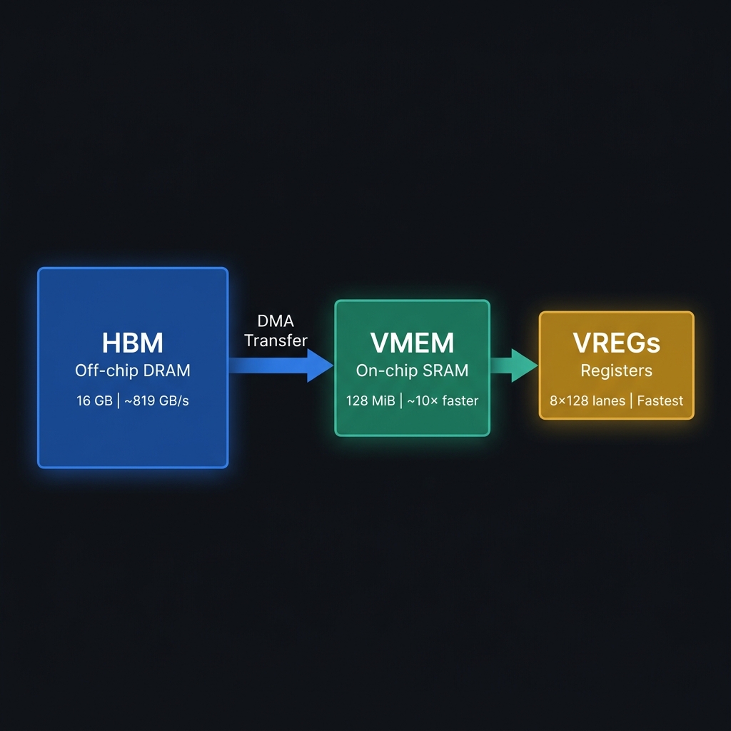
HBM  (16 GB, ~819 GB/s)  →  VMEM  (128 MiB, ~10× faster)  →  VREGs  (registers)
       Off-chip DRAM              On-chip SRAM                    Fastest

Level	What it is	TPU v5e size	Speed
HBM	High Bandwidth Memory. Where full tensors (Q, K, V, O) live.	16 GB	~819 GB/s bandwidth
VMEM	Vector Memory. On-chip SRAM scratchpad inside the TensorCore. Where Pallas tiles live during compute.	128 MiB	~10× faster than HBM
VREGs	Vector Registers. Where computation actually happens. Laid out as 8 sublanes × 128 lanes.	Small	Fastest

The key constraint: VMEM is fast but finite. Your block sizes, including double-buffered copies and scratch buffers, must fit within this budget. If they don’t, the Pallas compiler will either refuse to compile (VMEM overflow) or silently “spill” registers to VMEM, causing a severe performance cliff.

2.2 Compute Units

Unit	Purpose	Key fact
MXU (Matrix Multiply Unit)	Dense matrix multiplication	128×128 systolic array. Performs bf16 × bf16 → f32 accumulation natively. Peak: 197 TFLOP/s on v5e.
VPU (Vector Processing Unit)	Elementwise ops: add, mul, exp, max, comparisons, casts	Operates on vector registers. `exp` is medium cost; reductions over the last array dimension are the slowest path.
Scalar Unit	Control flow, loop indices, conditions	Used for grid orchestration — the `pl.program_id()` calls.

The MXU is a systolic array: weights are loaded into the grid of processing elements and held stationary, while activation data streams through row-by-row. Each of the 16,384 processing elements performs one multiply-accumulate per cycle. This massive parallelism is what gives TPUs their raw throughput on matrix operations — but the array must be saturated (inputs must be multiples of 128 in both dimensions) to achieve peak utilization.

2.3 The Roofline in One Sentence

Every kernel is either compute-bound (the MXU is the bottleneck; memory is fast enough to keep up) or memory-bound (the MXU is idle, waiting for data from HBM).

The dividing line is the ridge point, defined as:

[\text{Ridge Point} = \frac{\text{Peak FLOP/s}}{\text{Peak Bandwidth}} = \frac{197 \text{ TFLOP/s}}{819 \text{ GB/s}} \approx 240 \text{ FLOPs/byte}]

If your kernel’s arithmetic intensity (FLOPs per byte transferred) is above the ridge point, you’re compute-bound. Below it, you’re memory-bound. Most naive kernels — including naive attention — are deep in memory-bound territory.

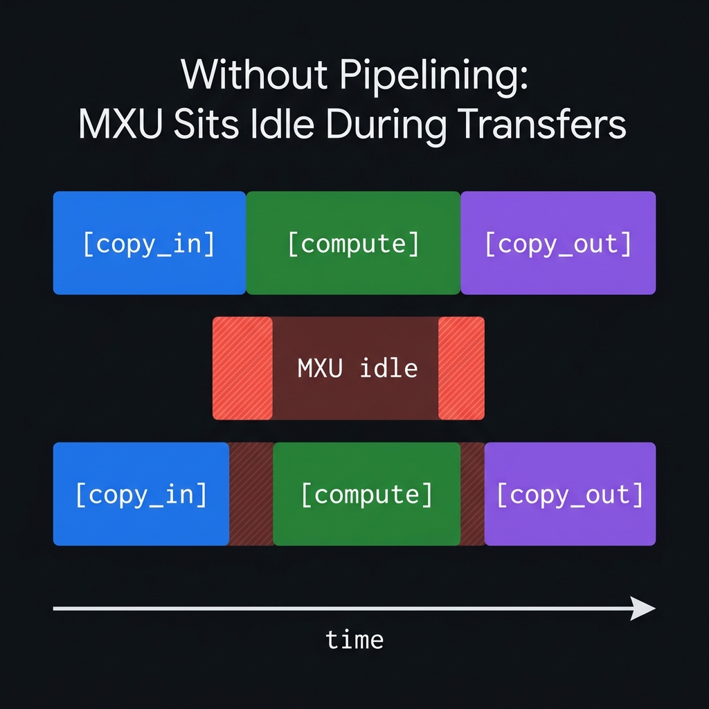
2.4 Double Buffering and Pipelining

The gap between HBM and VMEM speed is enormous. Without pipelining, the MXU sits idle during every DMA transfer:

[copy_in] [compute] [copy_out] [copy_in] [compute] [copy_out]
           idle ...                        idle ...

Pallas automatically uses double buffering: while one buffer is being used for compute, the next iteration’s data is being copied into a second buffer. In steady state, DMA and compute happen simultaneously:

[DMA 0]
        [DMA 1] [Compute 0]
                [DMA 2] [Compute 1] [DMA_out 0]
                        [Compute 2] [DMA_out 1]
                                    [DMA_out 2]

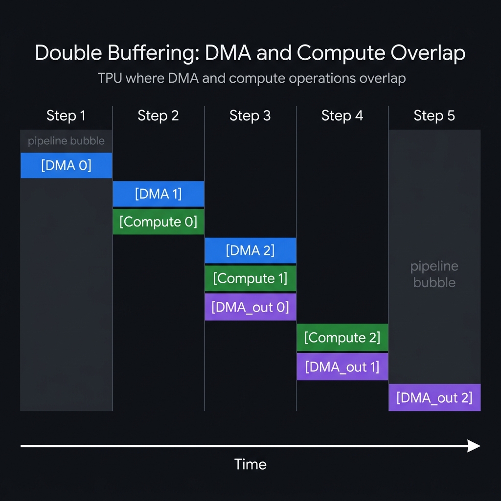
The first and last few steps — where not all pipeline stages are active — are called pipeline bubbles. More grid iterations mean a smaller bubble fraction, which means better efficiency.

3. The Pallas Programming Model

A Pallas kernel is built from four primitives. Every kernel you’ll ever write combines these four ideas.

3.1 Refs (Not Arrays)

Your kernel function doesn’t receive JAX arrays. It receives Refs — pointers to buffers in VMEM. You explicitly read from and write to them:

def my_kernel(x_ref, y_ref, o_ref):
    x = x_ref[...]         # Read: VMEM → VREGs
    y = y_ref[...]         # Read: VMEM → VREGs
    o_ref[...] = x + y     # Write: VREGs → VMEM

Input refs are read-only; output refs are write-only (except during accumulation patterns where you read and update in place via scratch buffers).

3.2 The Grid

The grid parameter defines how many times your kernel function is invoked:

grid = (num_q_blocks, num_kv_blocks)
# Equivalent to:
# for i in range(num_q_blocks):
#   for j in range(num_kv_blocks):
#     kernel(...)

A critical TPU difference: grid iterations run sequentially in lexicographic order, not in parallel like GPU thread blocks. This is exactly what makes accumulation patterns possible — you can keep an accumulator in VMEM across multiple iterations of the inner loop.

3.3 BlockSpecs — Mapping Grid Indices to Memory Slices

A BlockSpec tells Pallas which slice of the full HBM tensor to load into VMEM for each grid iteration:

pl.BlockSpec(
    block_shape=(BQ, HEAD_DIM),     # Shape of each tile
    index_map=lambda i, j: (i, 0)   # Maps grid indices → block indices
)

The index_map returns block indices, not element indices. The element index is block_index × block_size. For attention, we want Q tiles indexed by i and K/V tiles indexed by j:

pl.BlockSpec((BQ, d), lambda i, j: (i, 0))   # Q: the i-th query chunk
pl.BlockSpec((BKV, d), lambda i, j: (j, 0))  # K: the j-th key chunk
pl.BlockSpec((BKV, d), lambda i, j: (j, 0))  # V: the j-th value chunk

3.4 Scratch Memory — State That Persists Across Iterations

Scratch buffers live in VMEM and persist across grid iterations — they are not double-buffered. This makes them ideal for accumulators and running statistics:

scratch_shapes=[
    pltpu.VMEM((BQ, HEAD_DIM), jnp.float32),  # acc  — running output
    pltpu.VMEM((BQ, HEAD_DIM), jnp.float32),  # m    — running row-max
    pltpu.VMEM((BQ, HEAD_DIM), jnp.float32),  # l    — running row-sum
]

3.5 Putting It Together: `pallas_call`

result = pl.pallas_call(
    kernel_fn,                           # Your kernel function
    grid_spec=pltpu.PrefetchScalarGridSpec(
        num_scalar_prefetch=0,
        in_specs=[...],                  # BlockSpecs for inputs
        out_specs=...,                   # BlockSpec for output
        scratch_shapes=[...],            # Persistent VMEM buffers
        grid=(M, N),                     # Iteration space
    ),
    out_shape=jax.ShapeDtypeStruct(...), # Output shape/dtype
    compiler_params=pltpu.CompilerParams(
        dimension_semantics=("parallel", "arbitrary"),
    ),
)(q, k, v)

The dimension_semantics argument tells the Mosaic compiler which grid dimensions have cross-iteration dependencies:

"parallel": No dependencies — can be split across cores on multi-core TPUs (v4, v5p).
"arbitrary": Has dependencies (e.g., accumulation) — must run sequentially.

4. Naive Attention: The Starting Point

Before we build anything clever, let’s understand what we’re replacing. Here is standard attention, implemented in plain JAX:

def reference_fn(q, k, v):
    d = q.shape[-1]
    s = jnp.dot(q.astype(jnp.float32), k.astype(jnp.float32).T) / math.sqrt(d)
    p = jax.nn.softmax(s, axis=-1)
    return jnp.dot(p, v.astype(jnp.float32)).astype(jnp.bfloat16)

This is mathematically correct, numerically stable (the softmax is computed in f32), and trivially simple. It’s also catastrophically inefficient.

Why It’s Slow: The Memory Wall

At seq_len = 16,384 and head_dim = 128:

Q @ K^T produces a (16384, 16384) score matrix. In float32, that’s 16384² × 4 bytes = 1.07 GB.
This entire matrix is written to HBM, then read back for the softmax.
The softmax result P (16384² values) is written to HBM again, then read back for P @ V.
Total HBM traffic for intermediates alone: ~3.2 GB of round-trips.

The FLOPs are dominated by two matmuls: Q @ K^T and P @ V, totaling approximately 4 × seq² × d ≈ 137 GFLOP. The arithmetic intensity comes out to roughly:

[\text{Intensity} = \frac{137 \text{ GFLOP}}{3.2 \text{ GB}} \approx 43 \text{ FLOPs/byte}]

That’s 5.6× below the ridge point of 240 FLOPs/byte. The MXU is starved — it spends most of its time waiting for data to shuttle through HBM.

5. The FlashAttention Algorithm: Online Softmax

The core insight behind FlashAttention (Dao et al., 2022) is simple: never materialize the full attention matrix. Instead, process Q and K/V in tiles, computing partial softmax results and accumulating them using an online algorithm that maintains running statistics.

5.1 Why Standard Softmax Needs Two Passes

The standard softmax formula for a row $x = [x_1, \ldots, x_n]$ is:

[\text{softmax}(x_i) = \frac{e^{x_i - m}}{\sum_{j=1}^{n} e^{x_j - m}}, \quad m = \max(x)]

Computing this requires two passes over the data:

Pass 1: Find the maximum $m$.
Pass 2: Compute all $e^{x_j - m}$ and their sum.

For a full attention row, that means you need all $n$ score values before you can compute any softmax output. At $n = 16,384$, you’re forced to materialize the full row.

5.2 The Online Softmax Recurrence

The key observation is that you can update a partial softmax when new data arrives. Suppose you’ve processed KV blocks $1, \ldots, j{-}1$ and maintained:

$m^{(j-1)}$: running maximum of all scores seen so far (scalar per query row)
$l^{(j-1)}$: running sum of exponentials: $\sum_{i=1}^{(j-1) \cdot B_{KV}} e^{s_i - m^{(j-1)}}$
$O^{(j-1)}{\text{acc}}$: running output accumulator: $\sum{i=1}^{(j-1) \cdot B_{KV}} e^{s_i - m^{(j-1)}} \cdot V_i$

When the next KV block $j$ arrives, the update rules are:

[m^{(j)} = \max\left(m^{(j-1)},\; \max_k(S^{(j)}_k)\right)]

[\alpha = e^{m^{(j-1)} - m^{(j)}} \qquad \text{(correction factor)}]

[l^{(j)} = \alpha \cdot l^{(j-1)} + \sum_k e^{S^{(j)}_k - m^{(j)}}]

[O^{(j)}{\text{acc}} = \alpha \cdot O^{(j-1)}{\text{acc}} + P^{(j)} \cdot V^{(j)}]

where $P^{(j)}_k = e^{S^{(j)}_k - m^{(j)}}$ are the unnormalized attention weights for block $j$.

At the end, after all KV blocks are processed:

[O = \frac{O^{(\text{final})}_{\text{acc}}}{l^{(\text{final})}}]

5.3 Why This Works

The correction factor $\alpha$ rescales all previously accumulated values to the new maximum. This is mathematically exact — not an approximation. The final result is identical to the standard softmax-attention formula.

The critical advantage: only a (BQ, BKV) tile of scores lives in VMEM at any time. The accumulator O_acc is (BQ, d) — proportional to the block size, not the sequence length. The O(seq²) HBM allocation is eliminated entirely.

5.4 Mapping the Algorithm to the Kernel

Here is how the recurrence maps directly to our Pallas kernel body. Each kernel invocation processes one (q_block, kv_block) pair:

def attention_kernel(q_ref, k_ref, v_ref, o_ref, acc_ref, m_ref, l_ref, *, nsteps):
    kv_step = pl.program_id(1)

    # Initialize scratch on first KV step
    @pl.when(kv_step == 0)
    def _():
        acc_ref[...] = jnp.zeros((bq, d), dtype=jnp.float32)
        m_ref[...]   = jnp.full((bq, d), float("-inf"), dtype=jnp.float32)
        l_ref[...]   = jnp.zeros((bq, d), dtype=jnp.float32)

    # Load tiles from VMEM into registers
    q = q_ref[...]    # (BQ, d)
    k = k_ref[...]    # (BKV, d)
    v = v_ref[...]    # (BKV, d)

    # --- S = Q @ K^T ---
    s = lax.dot_general(q, k,
        dimension_numbers=(((1,), (1,)), ((), ())),
        preferred_element_type=jnp.float32)    # (BQ, BKV) in f32

    # --- Online softmax update ---
    block_max = jnp.max(s, axis=1)             # (BQ,)
    m_prev = m_ref[:, 0]                       # (BQ,) — extract from scratch
    m_new  = jnp.maximum(m_prev, block_max)    # (BQ,)
    alpha  = jnp.exp(m_prev - m_new)           # correction factor

    p = jnp.exp(s - m_new[:, None])            # (BQ, BKV) — unnormalized weights
    l_new = alpha * l_ref[:, 0] + jnp.sum(p, axis=1)

    # --- Accumulate: O_acc = alpha * O_acc + P @ V ---
    pv = lax.dot_general(p.astype(jnp.bfloat16), v,
        dimension_numbers=(((1,), (0,)), ((), ())),
        preferred_element_type=jnp.float32)    # (BQ, d) in f32

    acc_ref[...] = alpha[:, None] * acc_ref[...] + pv
    m_ref[...] = m_new[:, None] * jnp.ones((1, d), dtype=jnp.float32)
    l_ref[...] = l_new[:, None] * jnp.ones((1, d), dtype=jnp.float32)

    # --- Final normalization on last KV step ---
    @pl.when(kv_step == nsteps - 1)
    def _():
        o_ref[...] = (acc_ref[...] / l_ref[:, 0][:, None]).astype(jnp.bfloat16)

This is a working FlashAttention kernel, and it’s correct. But it has several deliberately naive choices that leave significant performance on the table. Understanding what’s naive — and what to do about it — is what the rest of this article is about.

6. What Is Kernel Fusion?

Before diving into specific optimizations, we need to define the concept that ties them all together: kernel fusion.

6.1 The Unfused World

In a standard JAX computation, each operation launches a separate kernel. For attention, the chain looks like:

QK matmul      →  write to HBM  →  read from HBM
Scale (/ √d)   →  write to HBM  →  read from HBM
Softmax (max → exp → sum → div)  →  write to HBM  →  read from HBM
PV matmul      →  write to HBM

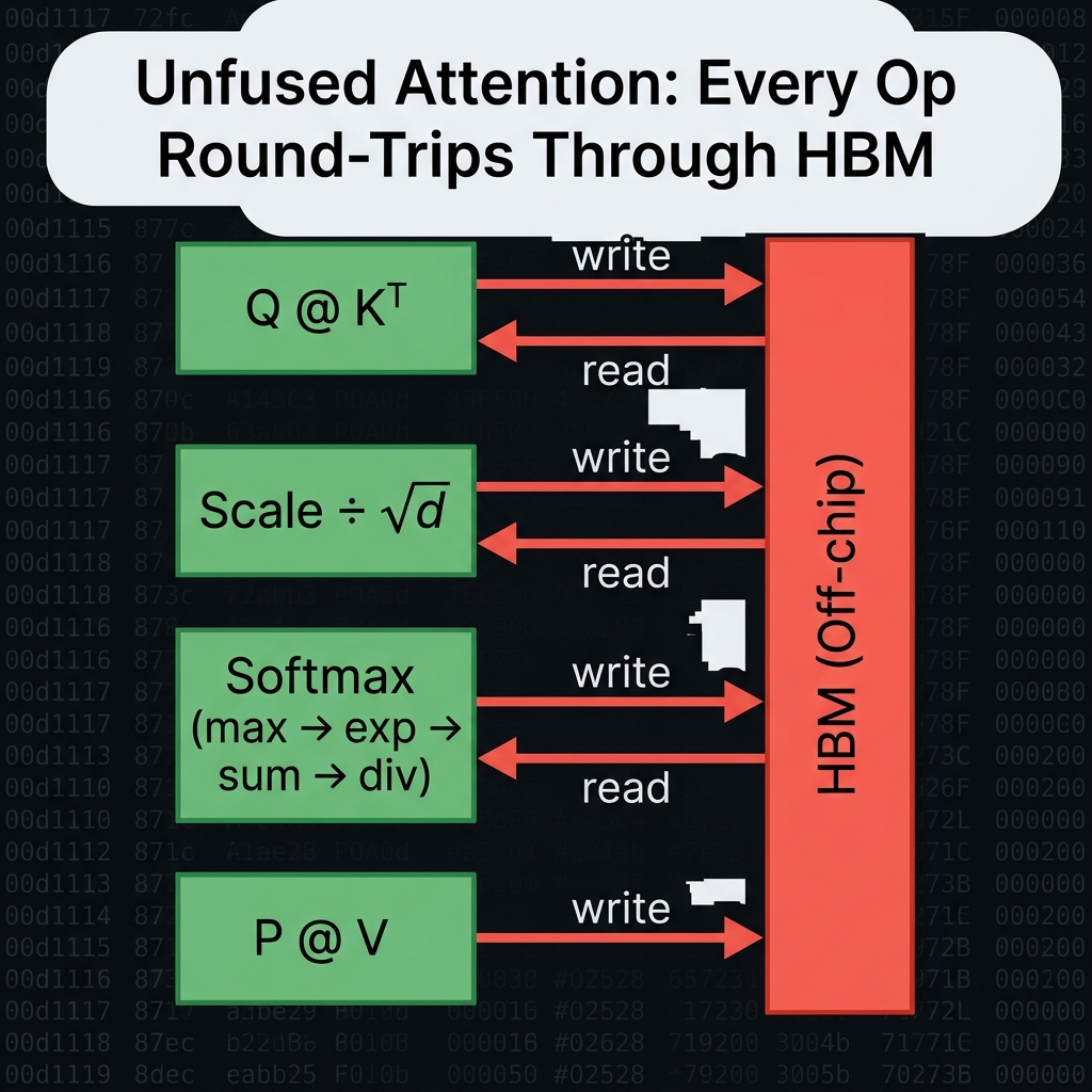
Each write → read round-trip through HBM is a bandwidth tax that delivers zero computational benefit. For elementwise operations like scaling and softmax, the compute cost is trivial compared to the memory traffic — these operations are inherently memory-bound.

6.2 The Fused World

In a fused kernel, all of the above happens in a single kernel launch. Intermediate values live in VMEM or VREGs and never touch HBM until the final output:

Tile loop (for each Q-block, for each KV-block):
    Load Q_i, K_j, V_j from HBM → VMEM         [once per tile]
    S = Q_i @ K_j^T                              [MXU, in VREGs]
    online softmax update (m, l, acc)             [VPU, in VREGs]
Write O_i from VMEM → HBM                        [once per Q-block]

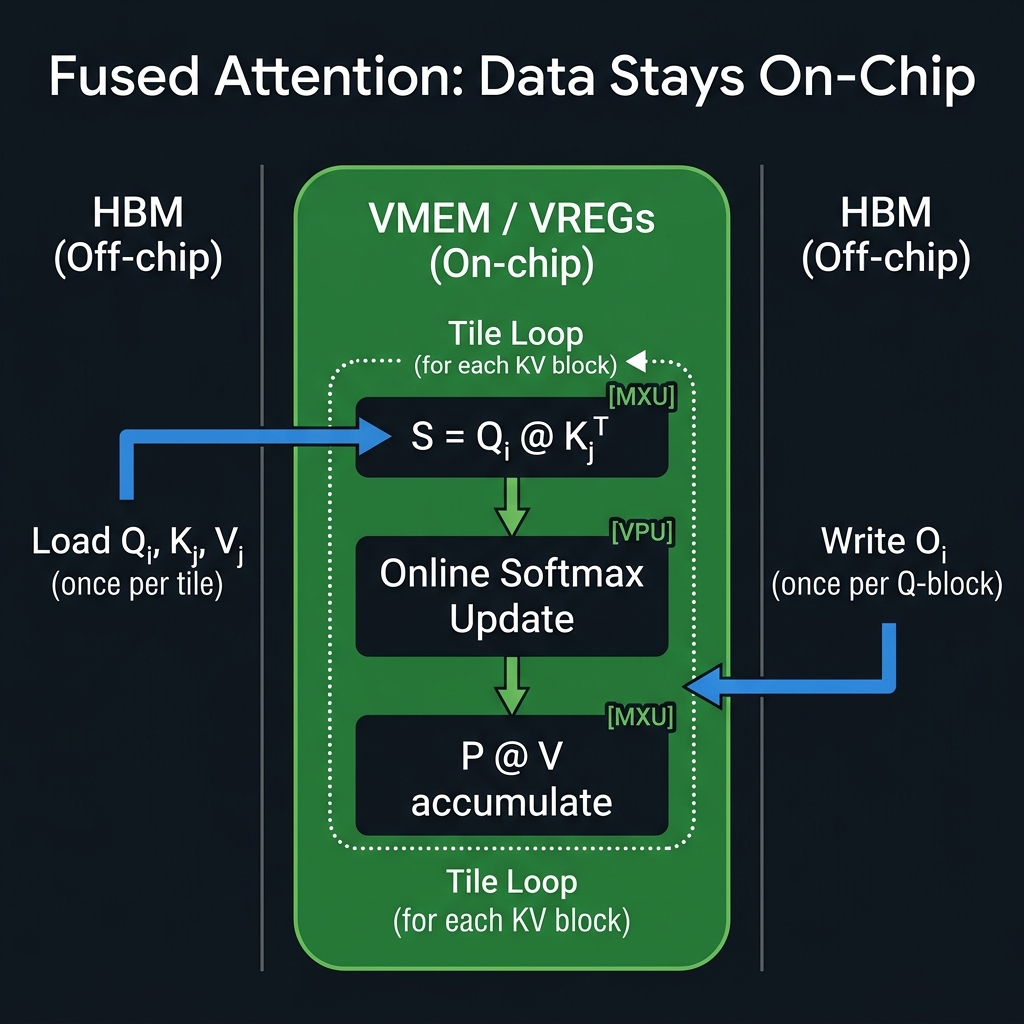
The total HBM traffic drops from O(seq² × multiple round-trips) to O(seq × d × small constant). This is the fundamental advantage of fusion.

6.3 The Fusion Spectrum: Inner Loop vs. Outer Loop

Not all fused computations are equal. Operations that run inside the inner KV loop execute once per tile, while operations in the outer loop execute once per Q-block:

Operation	Where it runs	Cost per Q-block
Scale Q by 1/√d	Outside the pallas_call (once total)	Free
Q @ K^T matmul	Inner loop (every KV step)	BQ × BKV × d MXU ops
exp(S − m)	Inner loop (every KV step)	BQ × BKV VPU ops
Row-wise max/sum	Inner loop (every KV step)	BQ × BKV VPU reductions
P @ V matmul	Inner loop (every KV step)	BQ × d × BKV MXU ops
Final O normalization	Inner loop (last KV step only)	BQ × d VPU ops

The takeaway: anything you can move from the inner loop to the outer loop — or outside the kernel entirely — is essentially free.

7. Fusion Experiments

Now let’s run concrete experiments. Each fusion targets a specific inefficiency in the naive kernel, and we measure the effect using the prepare.py benchmark harness.

Experiment A: Pre-Scale Q — Moving Invariant Work Outside the Loop

The Problem: In the naive kernel, the score matrix S needs to be scaled by $1/\sqrt{d}$. If this scaling is applied inside the inner loop, it costs BQ × BKV multiplications per KV step — and the same scale factor is applied identically every time.

The Fix: Move the scaling into the wrapper function, before the pallas_call:

def flash_attention(q, k, v, *, bq=BQ, bkv=BKV):
    seq_len, d = q.shape
    sm_scale = 1.0 / math.sqrt(d)
    q = q * sm_scale            # ← Scale once, outside the kernel
    nsteps = seq_len // bkv
    return pl.pallas_call(...)( q, k, v)

Inside the kernel, q_ref[...] now contains pre-scaled queries. The s *= scale line disappears entirely from the inner loop.

Why It Matters: At BQ=1024, BKV=512, and $d$=128, the kernel loop runs seq_len / BKV = 32 steps per Q-block. That’s 32 × 1024 × 512 = 16.7M multiply operations eliminated per Q-block. The total across all Q-blocks: 16 × 16.7M ≈ 268M floating-point operations removed. Not earth-shattering, but it’s free performance.

Result (placeholder):

Before:  latency=X.XXms  util=XX.X%  tflops=XXX.X
After:   latency=X.XXms  util=XX.X%  tflops=XXX.X

Experiment B: Precision Management — Let the MXU Do What It Does Best

The Problem: The naive kernel has several precision mistakes:

Q and K are bf16 tensors. The lax.dot_general with preferred_element_type=jnp.float32 tells the MXU to accumulate in f32 — which is correct. But if the inputs are upcast to f32 before the dot, the MXU still truncates them to bf16 internally (it’s a bf16 × bf16 systolic array on v5e). The upcast wastes bandwidth for zero accuracy gain.
V is similarly upcast to f32 unnecessarily before P @ V.
P (the softmax output, computed in f32) is cast to bf16 before the P @ V matmul. This discards softmax precision.

The Fix: Keep Q, K, V in their native bf16 and let preferred_element_type=jnp.float32 handle accumulation:

# Before (naive):
s = lax.dot_general(
    q.astype(jnp.float32),        # ← unnecessary upcast
    k.astype(jnp.float32),        # ← unnecessary upcast
    ..., preferred_element_type=jnp.float32)

# After (optimized):
s = lax.dot_general(
    q, k,                          # ← keep as bf16
    ..., preferred_element_type=jnp.float32)

Why It Matters: Keeping Q and K in bf16 halves the bandwidth required to load them from VMEM into VREGs for the matmul. The MXU natively processes bf16 inputs and accumulates in f32 — this is its designed operating mode. Forcing f32 inputs gains nothing arithmetically and costs double the memory traffic.

Result (placeholder):

Before:  latency=X.XXms  util=XX.X%  tflops=XXX.X
After:   latency=X.XXms  util=XX.X%  tflops=XXX.X

Experiment C: Compact Scratch Buffers — Eliminating 128× VMEM Waste

The Problem: The running maximum m and running sum l are scalars per query row — one value per row of the Q block. That’s BQ values each. But the naive kernel stores them as (BQ, HEAD_DIM) arrays with every column identical:

# Naive scratch shapes — 128× waste
pltpu.VMEM((BQ, HEAD_DIM), jnp.float32),  # m: (1024, 128) = 512 KB
pltpu.VMEM((BQ, HEAD_DIM), jnp.float32),  # l: (1024, 128) = 512 KB

At BQ=1024 and HEAD_DIM=128, each buffer is 1024 × 128 × 4 = 512 KB. The actual information content is 1024 × 4 = 4 KB — a 128× waste. This inflates both VMEM usage and the write traffic when updating m and l at every KV step.

The Fix: Store m and l as (BQ,) shaped scratch. Broadcast to (BQ, 1) only when needed for the rescale:

# Compact scratch shapes
pltpu.VMEM((BQ,), jnp.float32),  # m: (1024,) = 4 KB
pltpu.VMEM((BQ,), jnp.float32),  # l: (1024,) = 4 KB

And in the kernel body:

# Before:
m_ref[...] = m_new[:, None] * jnp.ones((1, d), dtype=jnp.float32)  # broadcast write

# After:
m_ref[...] = m_new          # direct scalar-per-row write

Why It Matters: This optimization saves 1 MB of VMEM (from 1024 KB to 8 KB for both m and l combined). More importantly, it eliminates 2 × BQ × HEAD_DIM × 4 bytes = 1 MB of VMEM writes per KV step. Over 32 KV steps per Q-block and 16 Q-blocks, that’s 32 × 16 × 1 MB = 512 MB of wasted write traffic eliminated.

Note: Whether (BQ,) shaped scratch works depends on the Pallas compiler version and TPU generation. The VPU register tile shape is 8 × 128, and scalar-per-row buffers may require special handling. If the compiler rejects this shape, the fallback is (BQ, 1) — still a 128× improvement over the naive approach.

Result (placeholder):

Before:  latency=X.XXms  util=XX.X%  tflops=XXX.X
After:   latency=X.XXms  util=XX.X%  tflops=XXX.X

8. The Full Fused Kernel

Incorporating all three fusions, the cleaned-up kernel looks like this:

BQ  = 1024   # Query block size
BKV = 512    # Key/Value block size

def attention_kernel(q_ref, k_ref, v_ref, o_ref, acc_ref, m_ref, l_ref, *, nsteps):
    kv_step = pl.program_id(1)
    bq, d = q_ref.shape

    @pl.when(kv_step == 0)
    def _():
        acc_ref[...] = jnp.zeros((bq, d), dtype=jnp.float32)
        m_ref[...]   = jnp.full((bq, d), float("-inf"), dtype=jnp.float32)
        l_ref[...]   = jnp.zeros((bq, d), dtype=jnp.float32)

    # Q is already pre-scaled by 1/sqrt(d) in the wrapper
    q = q_ref[...]    # bf16 — no upcast
    k = k_ref[...]    # bf16 — no upcast
    v = v_ref[...]    # bf16 — no upcast

    # S = Q_scaled @ K^T  — bf16 inputs, f32 accumulation
    s = lax.dot_general(q, k,
        dimension_numbers=(((1,), (1,)), ((), ())),
        preferred_element_type=jnp.float32)

    # Online softmax update
    block_max = jnp.max(s, axis=1)
    m_prev = m_ref[:, 0]
    m_new  = jnp.maximum(m_prev, block_max)
    alpha  = jnp.exp(m_prev - m_new)
    p      = jnp.exp(s - m_new[:, None])
    l_new  = alpha * l_ref[:, 0] + jnp.sum(p, axis=1)

    # P @ V — P in bf16, accumulate in f32
    pv = lax.dot_general(p.astype(jnp.bfloat16), v,
        dimension_numbers=(((1,), (0,)), ((), ())),
        preferred_element_type=jnp.float32)

    acc_ref[...] = alpha[:, None] * acc_ref[...] + pv
    m_ref[...] = m_new[:, None] * jnp.ones((1, d), dtype=jnp.float32)
    l_ref[...] = l_new[:, None] * jnp.ones((1, d), dtype=jnp.float32)

    @pl.when(kv_step == nsteps - 1)
    def _():
        o_ref[...] = (acc_ref[...] / l_ref[:, 0][:, None]).astype(jnp.bfloat16)


@functools.partial(jax.jit, static_argnames=["bq", "bkv"])
def flash_attention(q, k, v, *, bq=BQ, bkv=BKV):
    seq_len, d = q.shape
    q = q * (1.0 / math.sqrt(d))    # Pre-scale outside the kernel
    nsteps = seq_len // bkv
    return pl.pallas_call(
        functools.partial(attention_kernel, nsteps=nsteps),
        grid_spec=pltpu.PrefetchScalarGridSpec(
            num_scalar_prefetch=0,
            in_specs=[
                pl.BlockSpec((bq, d), lambda i, j: (i, 0)),
                pl.BlockSpec((bkv, d), lambda i, j: (j, 0)),
                pl.BlockSpec((bkv, d), lambda i, j: (j, 0)),
            ],
            out_specs=pl.BlockSpec((bq, d), lambda i, j: (i, 0)),
            scratch_shapes=[
                pltpu.VMEM((bq, d), jnp.float32),    # acc
                pltpu.VMEM((bq, d), jnp.float32),    # m
                pltpu.VMEM((bq, d), jnp.float32),    # l
            ],
            grid=(seq_len // bq, nsteps),
        ),
        out_shape=jax.ShapeDtypeStruct((seq_len, d), jnp.bfloat16),
        compiler_params=pltpu.CompilerParams(
            dimension_semantics=("parallel", "arbitrary"),
        ),
    )(q, k, v)

Benchmark summary (placeholder):

RESULT: score=XXXX.XX  latency=X.XXms  util=XX.XX%  tflops=XXX.XX
REGIME: COMPUTE-BOUND  BW=XX.X%  intensity=XXX FLOPs/byte

9. Takeaways

What we built: A single-head FlashAttention kernel in Pallas that computes exact attention without ever materializing the $n \times n$ score matrix in HBM. The kernel tiles the computation into (BQ, BKV) blocks, uses the online softmax recurrence to maintain running statistics in VMEM scratch buffers, and fuses all operations — scaling, matmuls, softmax, normalization — into a single kernel launch.

What we learned about fusion:

Moving invariant work (like Q scaling) outside the kernel loop is the simplest and highest-value fusion.
Precision management — keeping inputs in bf16 and relying on MXU’s native bf16 × bf16 → f32 accumulation — eliminates wasteful type conversions.
Memory layout (scratch buffer shapes) directly impacts VMEM pressure and write traffic. A 128× waste in scratch is a 128× waste in bandwidth.

What’s next: This kernel runs, and it’s correct. But how do we know why it’s fast or slow? How do we read the roofline analysis, interpret the HLO, and use XProf traces to diagnose the remaining efficiency gap? That’s the subject of Article 2.

Glossary

Term	Definition
HBM	High Bandwidth Memory. Off-chip DRAM, ~819 GB/s on v5e. Where full tensors live.
VMEM	Vector Memory. On-chip SRAM scratchpad, 128 MiB on v5e. Where Pallas tiles live during compute.
VREGs	Vector Registers. 8 sublanes × 128 lanes. Where computation happens.
MXU	Matrix Multiply Unit. 128×128 systolic array. Peak: 197 TFLOP/s (bf16) on v5e.
VPU	Vector Processing Unit. Elementwise operations.
Ridge Point	Arithmetic intensity threshold (~240 FLOPs/byte on v5e) separating memory-bound from compute-bound.
BQ, BKV	Block sizes for query and key/value tiles along the sequence dimension.
Pallas	JAX’s kernel-authoring extension for writing custom accelerator kernels.
FlashAttention	Tiled, IO-aware attention algorithm (Dao et al., 2022) using online softmax.
Fusion	Combining multiple operations into a single kernel launch to avoid intermediate HBM round-trips.

References

Dao, T., Fu, D.Y., Ermon, S., Rudra, A., & Ré, C. (2022). FlashAttention: Fast and Memory-Efficient Exact Attention with IO-Awareness. NeurIPS.
Jouppi, N.P., et al. (2023). TPU v4: An Optically Reconfigurable Supercomputer for Machine Learning with Hardware Support for Embeddings. ISCA.
JAX Team. Pallas: A JAX Kernel Language. https://jax.readthedocs.io/en/latest/pallas/
Milakov, M. & Gimelshein, N. (2018). Online normalizer calculation for softmax. arXiv:1805.02867.

Implementing a Fast Attention Fusion Kernel

Table of Contents

Writing Fast Attention on TPU — From Naive Kernel to Fused FlashAttention with Pallas

1. Why Pallas?

2. TPU Architecture: The Minimum Viable Mental Model

2.1 The Memory Hierarchy

2.2 Compute Units

2.3 The Roofline in One Sentence

2.4 Double Buffering and Pipelining

3. The Pallas Programming Model

3.1 Refs (Not Arrays)

3.2 The Grid

3.3 BlockSpecs — Mapping Grid Indices to Memory Slices

3.4 Scratch Memory — State That Persists Across Iterations

3.5 Putting It Together: `pallas_call`

4. Naive Attention: The Starting Point

Why It’s Slow: The Memory Wall

5. The FlashAttention Algorithm: Online Softmax

5.1 Why Standard Softmax Needs Two Passes

5.2 The Online Softmax Recurrence

5.3 Why This Works

5.4 Mapping the Algorithm to the Kernel

6. What Is Kernel Fusion?

6.1 The Unfused World

6.2 The Fused World

6.3 The Fusion Spectrum: Inner Loop vs. Outer Loop

7. Fusion Experiments

Experiment A: Pre-Scale Q — Moving Invariant Work Outside the Loop

Experiment B: Precision Management — Let the MXU Do What It Does Best

Experiment C: Compact Scratch Buffers — Eliminating 128× VMEM Waste

8. The Full Fused Kernel

9. Takeaways

Glossary

References

Tags

About Keshan Sanjaya Sodimana

Implementing a Fast Attention Fusion Kernel

Table of Contents

Writing Fast Attention on TPU — From Naive Kernel to Fused FlashAttention with Pallas

1. Why Pallas?

2. TPU Architecture: The Minimum Viable Mental Model

2.1 The Memory Hierarchy

2.2 Compute Units

2.3 The Roofline in One Sentence

2.4 Double Buffering and Pipelining

3. The Pallas Programming Model

3.1 Refs (Not Arrays)

3.2 The Grid

3.3 BlockSpecs — Mapping Grid Indices to Memory Slices

3.4 Scratch Memory — State That Persists Across Iterations

3.5 Putting It Together: pallas_call

4. Naive Attention: The Starting Point

Why It’s Slow: The Memory Wall

5. The FlashAttention Algorithm: Online Softmax

5.1 Why Standard Softmax Needs Two Passes

5.2 The Online Softmax Recurrence

5.3 Why This Works

5.4 Mapping the Algorithm to the Kernel

6. What Is Kernel Fusion?

6.1 The Unfused World

6.2 The Fused World

6.3 The Fusion Spectrum: Inner Loop vs. Outer Loop

7. Fusion Experiments

Experiment A: Pre-Scale Q — Moving Invariant Work Outside the Loop

Experiment B: Precision Management — Let the MXU Do What It Does Best

Experiment C: Compact Scratch Buffers — Eliminating 128× VMEM Waste

8. The Full Fused Kernel

9. Takeaways

Glossary

References

Tags

Share This Post

About Keshan Sanjaya Sodimana

You Might Also Like

The Art of Controlled Randomness: A Deep Dive into Sampling techniques in LLMs

3.5 Putting It Together: `pallas_call`