Deep-Dive into TPU Profiling — XProf, HLO, and the Roofline Model

Part 2 of the KernelForge series on writing, profiling, and optimizing custom TPU kernels in Python.

Google Cloud credits are provided for this project.

At the end of Article 1, we had a working fused FlashAttention kernel. It computes exact attention without materializing the full score matrix, and it incorporates three targeted fusions — pre-scaling, precision management, and improved scratch layout.

But “working” and “fast” are different things. Right now, our kernel runs — but how efficiently? Is the MXU sitting idle for half the execution time? Is the HBM bus saturated? Is the compiler silently inserting copies that waste bandwidth?

You can’t answer these questions by staring at source code. You need profiling tools: instruments that show you what the hardware is actually doing, microsecond by microsecond.

This article covers the complete profiling stack for TPU kernels: how to capture and read XProf traces, how to interpret the roofline model as a quantitative decision framework, and how to decode HLO compiler output. By the end, you’ll have a systematic protocol for diagnosing why a kernel is slow — not just that it’s slow.

This article builds on the fused FlashAttention kernel from the previous post and introduces the concepts behind a benchmarking harness to analyze and improve the performance of the kernel.

1. The Profiling Stack

When you run a Pallas kernel, it passes through several layers before reaching the hardware. Each layer generates observable output:

Your Pallas kernel (Python)
     ↓
JAX tracing → XLA/Mosaic compiler → HLO (High-Level Operations)
     ↓
TPU runtime / driver → Hardware performance counters
     ↓
XProf (profiling framework) → .xplane.pb trace files
     ↓
XProf standalone server (UI) → Trace Viewer, HLO Op Profile, Roofline Model, Memory Viewer

XProf is now a fully standalone tool. It no longer requires TensorBoard to function — you install it directly (pip install xprof), launch it as its own server, and point your browser at port 8791. TensorBoard still works if you prefer it: as long as xprof is installed, a “Profile” tab will appear in TensorBoard backed by the same XProf engine. But the standalone server is the recommended path and what we’ll use throughout this series.

Which Tool Answers Which Question

Question	Primary Tool
Am I compute-bound or memory-bound?	XProf Roofline Model
Which op type is dominating wall time?	XProf HLO Op Profile
Are DMA and compute overlapping?	XProf Trace Viewer
Is the compiler inserting defensive copies?	HLO dump + Graph Viewer
Is there a pipeline bubble?	XProf Trace Viewer (look for gaps)
Is there register spilling?	Roofline Gap + HLO copy/spill ops
What fraction of MXU time is active?	XProf Utilization Viewer

Understanding each tool in isolation is useful. Understanding how to combine them into a diagnosis is what makes you effective.

2. Setting Up the Profiling Pipeline

2.1 Installation

pip install xprof

If you’re on Python 3.12+ and hit ModuleNotFoundError: No module named 'pkg_resources', install an older setuptools first:

pip install "setuptools<70" && pip install xprof

pip install "protobuf>=5.29.0"

2.2 Capturing a Profile from `prepare.py`

The benchmark harness prepare.py captures an XProf trace automatically as part of its Step 5 analysis. XProf expects trace files in a specific directory structure — .xplane.pb files nested under plugins/profile/<session_name>/. JAX’s profiler writes this layout automatically when you point it at a log directory.

The idiomatic capture pattern uses the jax.profiler.trace context manager:

import jax
import os

def capture_profile(inputs):
    log_dir = "./profile_data"
    os.makedirs(log_dir, exist_ok=True)

    # Context manager API — cleaner than start_trace/stop_trace
    with jax.profiler.trace(log_dir):
        for _ in range(3):
            jax.block_until_ready(kernel_fn(*inputs))

Or equivalently with the explicit start/stop API:

jax.profiler.start_trace(log_dir)
for _ in range(3):
    jax.block_until_ready(kernel_fn(*inputs))
jax.profiler.stop_trace()

Several details matter here:

Warmup runs: The 5 warmup iterations in the benchmark phase (separate from the 3 profile iterations) ensure JAX’s JIT compilation is complete before we start measuring. The profiled runs capture steady-state execution only.
block_until_ready(): JAX computations are dispatched asynchronously. Without this call, timing would measure dispatch latency, not execution time. block_until_ready() forces Python to wait until the TPU has finished processing.
Output format: JAX writes .xplane.pb protocol buffer files to ./profile_data/plugins/profile/<timestamp>/. XProf reads this layout natively.

2.3 Viewing with the XProf Standalone Server

xprof --port=8791 ./profile_data

You’ll see output like:

Attempting to start XProf server:
  Log Directory: ./profile_data
  Port: 8791
  Worker Service Address: 0.0.0.0:50051
  Hide Capture Button: False
XProf at http://localhost:8791/ (Press CTRL+C to quit)

Open http://localhost:8791/ in a browser. Available traces appear in the Sessions dropdown on the left. Select a session, then use the Tools dropdown to navigate between Trace Viewer, HLO Op Profile, Roofline Model, and so on.

If running on a Cloud TPU VM, forward the port to your local machine first:

# On your local machine:
gcloud compute tpus tpu-vm ssh <tpu-name> -- -L 8791:localhost:8791

# On the TPU VM:
xprof --port=8791 ./profile_data

TensorBoard compatibility: If you have an existing TensorBoard workflow, it continues to work unchanged. As long as xprof is installed, tensorboard --logdir=./profile_data will surface a Profile tab with identical functionality. XProf supersedes the old tensorboard-plugin-profile package — uninstall the latter if you have both.

2.4 Controlling What Gets Traced with `ProfileOptions`

XProf exposes fine-grained control over which hardware layers are captured via jax.profiler.ProfileOptions. This is important for TPU kernels because the default trace mode (TRACE_ONLY_XLA) captures XLA-level ops but not lower-level compute and DMA events. To see MXU activity and DMA transfers in the Trace Viewer, you need TRACE_COMPUTE:

import jax

options = jax.profiler.ProfileOptions()
options.advanced_configuration = {
    "tpu_trace_mode": "TRACE_COMPUTE_AND_SYNC"
}

jax.profiler.start_trace("./profile_data", profiler_options=options)
for _ in range(3):
    jax.block_until_ready(kernel_fn(*inputs))
jax.profiler.stop_trace()

Available tpu_trace_mode values and what they expose:

Mode	Captures
`TRACE_ONLY_HOST`	CPU/host activity only. No device traces.
`TRACE_ONLY_XLA`	XLA-level op graph on the device. Default if not specified.
`TRACE_COMPUTE`	Compute ops (MXU/VPU) on-device. Use this for kernel optimization.
`TRACE_COMPUTE_AND_SYNC`	Compute + synchronization events. Most detailed; use for debugging pipeline stalls.

For most kernel profiling work, TRACE_COMPUTE is the right setting. TRACE_COMPUTE_AND_SYNC is the setting to reach for when you suspect pipeline bubbles or DMA/compute scheduling issues.

To reduce noise from Python overhead and keep the trace focused on device activity:

options = jax.profiler.ProfileOptions()
options.python_tracer_level = 0    # disable Python function call tracing
options.host_tracer_level = 1      # only user-instrumented events on host
options.device_tracer_level = 1    # enable device tracing (default, make explicit)
options.advanced_configuration = {"tpu_trace_mode": "TRACE_COMPUTE"}

2.5 Manual Capture via the XProf UI (Long-Running Programs)

For training loops and other long-running programs where you want to trigger a profile capture at a specific point, XProf supports a server-based capture mode:

Add a profiler server to your program:

import jax.profiler
jax.profiler.start_server(9999)

Start the XProf UI:

xprof --logdir ./profile_data

In the browser at http://localhost:8791/, click Capture Profile. Enter localhost:9999 as the profile service URL, set the duration in milliseconds, and click Capture.

This lets you grab a profile snapshot while the kernel is executing inside a training step, without modifying the training loop itself.

2.6 Continuous Profiling Snapshots

XProf also supports a programmatic continuous profiling API, which is useful for capturing anomalous runs or debugging transient regressions without restarting:

from xprof.api import continuous_profiling_snapshot

# Start continuous profiling (connects to the running profiler server at port 9999)
continuous_profiling_snapshot.start_continuous_profiling('localhost:9999', {})

# ... run your workload ...

# Capture a snapshot at any moment
continuous_profiling_snapshot.get_snapshot('localhost:9999', './profile_data/')

# Stop
continuous_profiling_snapshot.stop_continuous_profiling('localhost:9999')

Then view it with:

xprof --port=8791 ./profile_data

In the kernelforge harness, the --deep flag activates this extended profiling mode:

./ratchet.sh "experiment: scratch buffer fix --deep"

Save it for when you need detailed before/after comparisons or are debugging transient regressions — it adds overhead and generates larger trace files.

2.7 Adding Custom Trace Annotations

By default, the Trace Viewer shows low-level internal JAX/XLA events. To annotate your own operations for easier identification in the timeline, use jax.profiler.TraceAnnotation:

import jax

with jax.profiler.trace("./profile_data"):
    for step in range(num_steps):
        with jax.profiler.TraceAnnotation(f"kernel_step_{step}"):
            jax.block_until_ready(kernel_fn(*inputs))

Or the decorator form for named functions:

@jax.profiler.annotate_function
def kernel_fn(*inputs):
    ...

These annotations appear as named spans in the Trace Viewer, making it straightforward to locate your kernel’s execution within a larger program timeline.

3. The Roofline Model — A Decision Framework

The roofline model is the most important analytical tool for kernel optimization. It tells you whether your bottleneck is compute or memory, and by how much.

XProf now includes a built-in Roofline Model tool, available under the Tools dropdown in any session. It plots your kernel’s measured performance directly on the roofline chart, eliminating the need to compute it manually for standard ops.

3.1 The Roofline Chart

The roofline plots achievable performance (TFLOP/s) against arithmetic intensity (FLOPs/byte):

Roofline

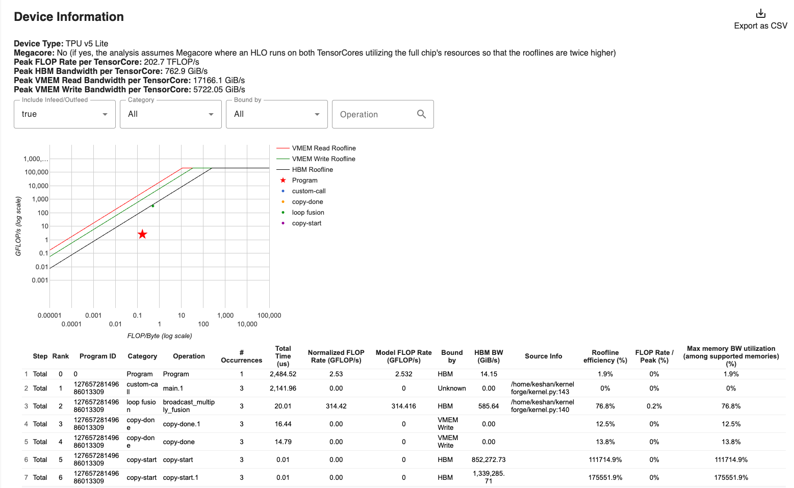
Left of the ridge point (intensity < 240): You’re memory-bound. The MXU can process data faster than HBM can deliver it. Performance is limited by bandwidth.
Right of the ridge point (intensity > 240): You’re compute-bound. HBM can deliver data faster than the MXU can consume it. Performance is limited by FLOP/s.

The ridge point for TPU v5e is:

$$\text{Ridge} = \frac{197 \times 10^{12} \text{ FLOP/s}}{819 \times 10^{9} \text{ B/s}} \approx 240 \text{ FLOPs/byte}$$

3.2 How `prepare.py` Computes Each Number

The harness outputs a summary line like:

RESULT: score=847.3  latency=2.12ms  util=64.8%  tflops=127.4
REGIME: COMPUTE-BOUND  BW=38.2%  intensity=682 FLOPs/byte

Here’s what each field means and how it’s calculated:

Field	Formula	Interpretation
`tflops`	`compute_flops() / median_latency`	Actual throughput achieved
`util`	`tflops / 197`	Fraction of the MXU’s theoretical peak
`intensity`	`compute_flops() / estimated_bytes_transferred`	Where you sit on the roofline
`BW%`	`bytes_transferred / (latency × 819 GB/s)`	Fraction of HBM bandwidth used
`score`	`util × 100 / latency`	Combined fitness metric for the ratchet loop

The compute_flops() function in kernel.py returns the theoretical FLOPs for the operation. For single-head attention at seq=16384, d=128:

Q@K^T:    2 × 16384² × 128 = 68.7 GFLOP
P@V:      2 × 16384² × 128 = 68.7 GFLOP
softmax:  ~5 × 16384²       =  1.3 GFLOP
Total:    ~138.8 GFLOP

The estimate_actual_memory_traffic() function uses tiling metadata from get_tiling_meta() to estimate total HBM bytes, including re-reads caused by the tiling pattern. For attention, K and V are re-read once per Q-block:

Q:  seq × d × 2 bytes × 1 re-read  =   4.0 MB
K:  seq × d × 2 bytes × num_q_blocks = 64.0 MB  (re-read per Q block)
V:  seq × d × 2 bytes × num_q_blocks = 64.0 MB
O:  seq × d × 2 bytes × 1 write    =   4.0 MB
Total: ~136 MB

At 136 MB traffic and 138.8 GFLOP: intensity ≈ 1020 FLOPs/byte — well above the ridge point of 240, so the kernel is compute-bound.

3.3 The Gap — The Most Informative Metric

The roofline gives two theoretical floors — the minimum time if only one resource were the bottleneck:

Compute-only time: compute_flops / peak_FLOPS = 138.8G / 197T = 0.70 ms
Memory-only time:  bytes_transferred / peak_BW = 136M / 819G  = 0.17 ms
Actual time:       measured median latency      =               2.12 ms

The Gap is defined as:

«divdiv> $\text{Gap} = \text{Actual} - \max(\text{Compute-only}, \text{Memory-only})$ </div>

In this example: 2.12 - 0.70 = 1.42 ms. A large gap means something beyond raw compute and memory access is consuming time. The likely culprits, in order of probability:

Register spilling: The score matrix (BQ × BKV) is too large for VREGs. When registers overflow, the compiler silently generates loads and stores to VMEM — adding traffic that neither the FLOP count nor the traffic estimate accounts for.
Pipeline bubbles: DMA and compute are not fully overlapping. This happens when the pipeline is too short (too few grid iterations) or when the compiler can’t schedule DMA and compute concurrently.
Defensive copies: The compiler inserts copy operations when it detects potential aliasing between input and output refs. Each copy is a full-buffer read+write that wastes bandwidth.
VPU bottleneck: If elementwise operations (exp, reduce) are slow enough to stall the MXU between matmul steps, you lose pipeline throughput even though you’re technically “compute-bound.”

3.4 Worked Example: Diagnosing a Memory-Bound Baseline

Here’s real-looking output from an early version of the kernel with small block sizes (BQ=128, BKV=256):

Bottleneck:          MEMORY-BOUND
Operational intensity:
    Actual (with re-reads): 85.3 FLOPs/byte
    Minimum (perfect reuse): 2730.7 FLOPs/byte
    Chip ridge point:        240.5 FLOPs/byte
  2.8x below ridge point
Memory traffic:
    Min (theoretical):  6.0 MB
    Est (with tiling):  1.6 GB
Time decomposition:
    Compute-only:  0.70 ms (if 100% MXU)
    Memory-only:   2.01 ms (if 100% BW)
    Actual:        5.20 ms
    Gap:           3.19 ms
Bandwidth:
    Achieved:      307.7 GB/s / 819 GB/s (37.6%)

Step-by-step diagnosis:

Regime: Memory-bound, 2.8× below ridge. The MXU is idle most of the time.
Actual vs. minimum intensity: 85 vs. 2731 FLOPs/byte. This is a 32× gap, meaning the tiling pattern causes K and V to be re-read ~32 times more than the theoretical minimum. With BQ=128 and seq=16384, there are 128 Q-blocks — K/V are re-read 128 times each.
Gap: 5.20 - 2.01 = 3.19 ms. Even if we could use 100% of HBM bandwidth, the kernel would still take 2.01 ms. The extra 3.19 ms suggests pipeline bubbles (128 × 64 = 8192 grid iterations is actually quite many, so the issue is more likely fragmented transfers and small tiles) or register pressure.
Bandwidth: Only 37.6% — the memory bus isn’t even saturated. The DMA transfers are too small to amortize the per-transfer overhead.

Prescription: Increase block sizes (BQ first, then BKV) to:

Reduce the number of Q-blocks → fewer K/V re-reads → higher intensity
Increase per-transfer size → better bandwidth utilization
Move toward the ridge point

4. XProf Trace Viewer — Reading the Timeline

The Trace Viewer shows a microsecond-level timeline of everything the TPU does. Learning to read it is the highest-leverage profiling skill.

Navigate there via: Sessions dropdown → [your session] → Tools → Trace Viewer. Use WASD to pan and zoom. Click or drag to select events for detailed stats.

4.1 What You See

The trace displays several rows:

Row: "Fused Ops"    — Compute operations on the MXU/VPU (your matmuls, exp, etc.)
Row: "Custom Calls"  — DMA transfers between HBM and VMEM
Row: "Host"          — Python/JAX dispatch on the CPU

TPU Trace Viewer

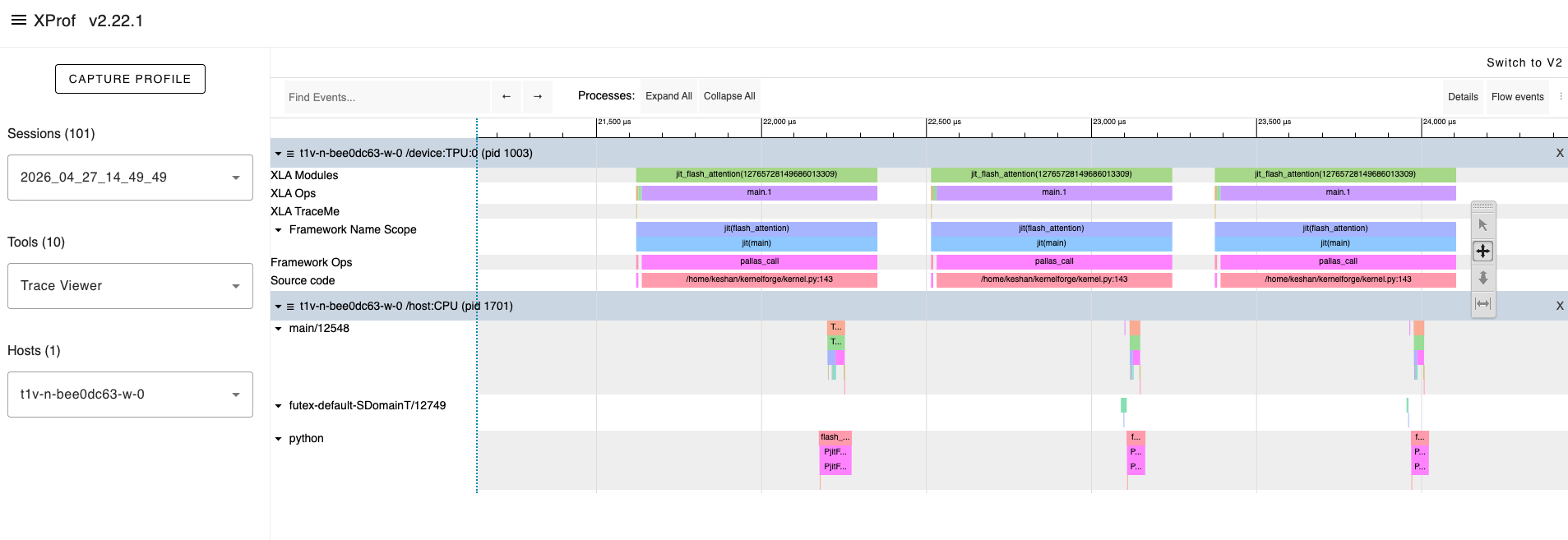
Each row contains blocks representing operations, with time progressing left to right.

Note: If these rows are sparse or missing, you may need to re-capture with tpu_trace_mode: "TRACE_COMPUTE" in your ProfileOptions. The default TRACE_ONLY_XLA mode doesn’t surface DMA and compute as separate rows.

4.2 Healthy vs. Unhealthy Patterns

Healthy (compute and DMA overlapping):

In steady state, you want to see DMA transfers and compute operations happening at the same time — stacked vertically in the timeline:

DMA:     [DMA_0] [DMA_1] [DMA_2] [DMA_3] [DMA_4] ...
Compute:         [Comp_0] [Comp_1] [Comp_2] [Comp_3] ...

The DMA for step $n+1$ happens concurrently with compute for step $n$. No idle time.

Unhealthy (pipeline bubble):

If you see horizontal gaps between compute blocks, the MXU was idle — waiting for data:

DMA:     [DMA_0]         [DMA_1]         [DMA_2]
Compute:         [Comp_0]        [Comp_1]        [Comp_2]
                    ^^^^            ^^^^
                   bubbles       (MXU idle)

This pattern indicates that DMA transfers are not being overlapped with compute. Common causes:

Block sizes are too small (DMA completes before compute, but there’s scheduling overhead between steps)
Double buffering isn’t active (check that you’re using PrefetchScalarGridSpec)
The pipeline is too short (too few grid iterations for the startup/drain cost to amortize)

4.3 Pattern Recognition Checklist

What you see	What it means	Action
White gaps between Fused Op blocks	Pipeline bubbles — MXU idle	More grid iterations, or increase block sizes
DMA not overlapping compute	Double buffering disabled or broken	Verify `PrefetchScalarGridSpec`; check in_specs/out_specs
Many very short Fused Op blocks	Block sizes too small — insufficient per-step work	Increase tile dimensions
One very long Fused Op block	Good MXU saturation per step	Check enough iterations for pipeline amortization
`copy` events in the timeline	Defensive copies from aliasing	Inspect HLO for unnecessary copies; refactor scratch buffer usage
Long gaps at the start and end	Pipeline fill and drain (“bubbles”)	Normal if grid is small. Increase grid iterations to reduce the fraction

4.4 How to Read the Trace Step-by-Step

Zoom to the steady-state region: Ignore the first 2–3 compute blocks (pipeline fill) and the last 2–3 (pipeline drain). Use WASD to zoom in on the middle.
Check DMA/compute overlap: In the steady-state region, DMA blocks should appear above compute blocks at the same horizontal position. If they’re sequential, pipelining is broken.
Count the Fused Op blocks: The total should equal your grid dimension product. For attention with BQ=1024, BKV=512, seq=16384: (16384/1024) × (16384/512) = 16 × 32 = 512 blocks.
Measure the bubble fraction: bubble_time / total_time. Anything above 10% is a red flag. Below 5% is excellent.
Check for copy events: These appear as short blocks between compute blocks. Each copy is a full-buffer read+write that wastes bandwidth. Their presence in steady state means the compiler detected aliasing.

4.5 The HLO Op Profile View

The HLO Op Profile (in the Tools dropdown) shows aggregate time spent per operation type across the entire capture. This answers: “which operation type is dominating wall time?”

Key things to look for:

exponential (exp) dominating: This is a VPU bottleneck. The softmax’s exp operations are slowing the inner loop. The MXU finishes its matmul and then waits for the VPU to finish the exponentiation before the next P@V matmul can proceed.
reduce (max, sum) taking significant time: The row-wise reductions in online softmax reduce over the last array dimension (axis=1 of the (BQ, BKV) score matrix), which is the slowest reduction path on TPU. Consider transposing the score matrix to reduce over the second-to-last dimension instead.
Unexpected reshape, transpose, slice ops: The compiler is performing layout coercion — rearranging data to match the VPU/MXU’s expected input layout. This can indicate that your block shapes don’t align with the 8×128 VREG tile shape.

4.6 The Utilization Viewer

The Utilization Viewer translates raw hardware counters into percentages for each unit:

TC% (TensorCore / MXU): Fraction of time the MXU is doing useful matmuls. This is the number you want to maximize.
HBM read/write %: Fraction of time the HBM bus is actively transferring data.

Key interpretation:

TC%	HBM%	Meaning
High	Low	Compute-bound, efficient — ideal for matmul-heavy kernels
Low	High	Memory-bound — increase intensity
Low	Low	Pipeline bubbles or overhead — neither unit is being utilized
High	High	Good overlap — you’re approaching the hardware ceiling

5. HLO Analysis — What the Compiler Actually Generates

5.1 What Is HLO?

HLO (High-Level Operations) is XLA’s intermediate representation — the computation graph that describes exactly what the TPU will execute, after all JAX transformations (tracing, jit compilation, fusion) but before hardware-specific lowering.

For Pallas kernels, the path is: Pallas Python → Mosaic IR → XLA → HLO → LLO (Low-Level Operations) → TPU machine code.

HLO is the last representation that’s readable by humans. XProf exposes it through two complementary interfaces:

Graph Viewer (Tools → Graph Viewer): an interactive node-and-edge visualization of the HLO computation graph
Text dump (./profile_data/kernel.hlo.txt): the raw text file written by prepare.py

5.2 Finding and Reading the HLO Dump

prepare.py saves the HLO text to ./profile_data/kernel.hlo.txt and prints summary statistics:

HLO stats:
    dot ops:     2     ← one for QK^T, one for PV
    exp ops:     3     ← exp(m_prev - m_new), exp(s - m_new), possibly duplicated
    reduce ops:  4     ← max(s), sum(p), and perhaps compiler-inserted reductions
    copy ops:    1     ← ⚠️ investigate
    total lines: 847
    Full HLO:    ./profile_data/kernel.hlo.txt

5.3 What Each Counter Means

HLO Op	Expected Count	If Higher Than Expected
`dot`	2 (QK^T + PV)	The compiler is splitting your matmul into smaller pieces — block shapes may not align with MXU tile (128×128)
`exponential`	2 (block exp for softmax)	Redundant exp ops — check if the compiler is duplicating computation
`reduce`	2–4 (max + sum for softmax, possibly along different axes)	The compiler is decomposing your reduction into multiple stages
`copy`	0 (ideal)	Defensive copies — the compiler detected potential aliasing. See §5.4

5.4 Copy Ops — The Silent Performance Killer

Copy operations are the most actionable finding in HLO analysis. The compiler inserts them when two refs potentially alias the same buffer — particularly when an output ref is read and written in the same kernel body.

Common cause in Pallas: Using o_ref[...] as an accumulator (reading and writing the output ref mid-loop) without using a dedicated scratch buffer.

How to spot them: Open ./profile_data/kernel.hlo.txt and search for copy(:

%copy.63 = f32[1024,128]{1,0} copy(f32[1024,128]{1,0} %some_buffer.62)

Alternatively, use the Graph Viewer in XProf to visually locate copy nodes — they appear as standalone nodes in the data flow graph between the read and write operations.

Each copy is a full-buffer read+write. For a (1024, 128) f32 buffer, that’s 1024 × 128 × 4 = 512 KB of wasted traffic per copy, per grid iteration. Over 512 iterations, that’s 262 MB of unnecessary traffic.

Fix: Use dedicated scratch_shapes for all accumulators. Never read from an output ref before the final write.

5.5 Register Pressure — The Invisible Wall

Register spilling does not appear directly in HLO — it happens at the LLO (Low-Level Operations) layer, below what HLO exposes. But you can infer it from observable symptoms:

The smoking gun: The Gap metric (§3.3) suddenly increases when you increase BKV, even though VMEM usage is well within budget and the kernel is compute-bound.

The physics: The attention score matrix S = (BQ, BKV) in f32 occupies:

VREGs for S = BQ × BKV × 4 bytes

At BQ=1024, BKV=512: 1024 × 512 × 4 = 2 MB of register space just for the score matrix. When VREGs overflow, the Mosaic compiler generates implicit loads and stores to VMEM — these don’t appear as explicit copy ops in HLO but show up as increased VMEM traffic in the Trace Viewer.

Diagnosis tool: If you increase BKV and see a sudden nonlinear jump in latency (the “spill cliff”), you’ve exceeded the register budget. The correct action is to back off BKV to the last good value and look for gains elsewhere.

6. The Profiling Protocol — A Systematic Workflow

Here is a step-by-step protocol you can follow with any Pallas kernel. Print this, tape it to your monitor, and follow it every time.

Step 1: Capture the Baseline

Run prepare.py and record the summary line:

score=___  latency=___ms  util=___%  tflops=___
REGIME: ___  BW=___%  intensity=___ FLOPs/byte

Capture with TRACE_COMPUTE_AND_SYNC for maximum detail.

Step 2: Read the Roofline

Use XProf’s built-in Roofline Model tool (Tools → Roofline Model) to verify the regime classification. Then determine direction:

Memory-bound: Focus on reducing HBM traffic (larger blocks, fewer re-reads, better tiling)
Compute-bound: Focus on reducing per-step VPU work, improving MXU feeding, or algorithmic improvements (block skipping)

Calculate the Gap:

Gap = actual - max(compute_only, memory_only)
Small Gap (< 10% of actual): You’re near the roofline. Gains will be incremental.
Large Gap (> 30% of actual): Significant overhead — register spills, pipeline bubbles, or defensive copies.

Step 3: Check the HLO

cat ./profile_data/kernel.hlo.txt | grep -c "copy("

If copy_count > 0: Investigate aliasing in scratch buffers. Cross-check with Graph Viewer in XProf. If dot_count > expected: The compiler is splitting matmuls — check block shapes. If exp_count is high: VPU softmax overhead — can you simplify the math?

Step 4: Open the Trace Viewer

xprof --port=8791 ./profile_data
# Navigate to Sessions → [your session] → Tools → Trace Viewer

Find the steady-state region (skip first and last few iterations)
Check DMA/compute overlap (requires TRACE_COMPUTE or TRACE_COMPUTE_AND_SYNC)
Measure bubble fraction
Look for copy events

Step 5: Check the HLO Op Profile

Which op type dominates?
Is exp > 10% of total time → VPU bottleneck
Are there unexpected layout ops → block shape alignment issue

Step 6: Check Utilization

TC% high, HBM% low → compute-bound, good
Both low → pipeline bubbles or overhead dominating
HBM% high, TC% low → memory-bound, need higher intensity

Step 7: Form a Hypothesis

A good hypothesis is specific, testable, and tied to a profiling observation:

✅ “The roofline shows memory-bound with BW at 37%. Increasing BQ from 128 to 512 should reduce K/V re-reads by 4×, pushing intensity above the ridge point.”

❌ “Make it faster.”

Step 8: Make ONE Change

Never change two things at once. This is the isolation principle that makes results attributable.

Step 9: Repeat

Run prepare.py again. Compare the new summary to the baseline. Did the hypothesis hold? If yes, lock in the gain. If no, revert and form a new hypothesis.

7. Applying the Protocol: A Walk-Through

Let’s apply the protocol to our Flash Attention kernel from Article 1.

Starting Point

score=847.3  latency=2.12ms  util=64.8%  tflops=127.4
REGIME: COMPUTE-BOUND  BW=38.2%  intensity=682 FLOPs/byte
Gap: 1.42ms
HLO: 2 dots, 3 exps, 4 reduces, 1 copy

Step 2: Roofline

Compute-bound — good. But util is only 64.8%, meaning 35% of MXU time is wasted. The Gap of 1.42 ms (67% of actual) is substantial — there’s significant overhead beyond raw compute. XProf’s Roofline Model tool will plot our kernel’s point clearly left of where it should be relative to the compute ceiling at 197 TFLOP/s.

Step 3: HLO

One copy op. This shouldn’t be there if scratch buffers are correctly separated. The copy costs BQ × HEAD_DIM × 4 bytes = 512 KB per iteration, across 512 iterations = 262 MB of wasted traffic. Use the Graph Viewer to find which node the copy feeds — is it flowing into the matmul or the reduce?

Step 4: Trace Viewer

Captured with TRACE_COMPUTE_AND_SYNC. In the steady-state region, look for:

Visible gaps: Pipeline isn’t fully hiding DMA latency. With 512 grid iterations, the bubble fraction should be small — check.
Copy blocks between compute blocks: Confirms the HLO copy finding.

Step 5: HLO Op Profile

If exp contributes ~12% of total time, the VPU softmax operations are a secondary bottleneck. The exp runs once per KV step, computing BQ × BKV = 1024 × 512 = 524,288 exponentials per step.

Step 6: Utilization

TC (MXU) at 65%, HBM at 38%. The MXU is active 65% of the time. The other 35% is split between VPU work (exp, reduces), pipeline overhead, and the copy op.

Step 7: Hypotheses

Two hypotheses, in priority order:

“The copy op from scratch aliasing wastes ~262 MB of traffic. Eliminating it by fixing scratch buffer management should close ~10% of the gap.”
“The (BQ, HEAD_DIM) shaped m/l scratch buffers cause 128× unnecessary write traffic. Compacting them should reduce per-step VMEM writes and close additional gap.”

Step 8: Execute

Fix the copy op first (higher expected impact), then re-profile to see if the second hypothesis is still relevant.

8. Advanced XProf Features

8.1 Distributed Profiling

For multi-chip or multi-host workloads, XProf supports a distributed mode with separate aggregator and worker instances:

# Worker nodes (run on each TPU host):
xprof --grpc_port=50051

# Aggregator (your viewing machine):
xprof --port=8791 --worker_service_address=host1:50051,host2:50051 ./profile_data

This collects and correlates traces across all TPU chips simultaneously — essential for diagnosing cross-chip communication bottlenecks in multi-host training runs.

8.2 GCS Integration

XProf reads directly from Google Cloud Storage. If your training runs write profiles to a GCS bucket, you can view them without downloading:

xprof --port=8791 gs://your-bucket/profile_data

You can also dynamically load sessions without restarting the server by passing session_path or run_path as URL parameters in the browser:

http://localhost:8791/?session_path=gs://your-bucket/profile_data/plugins/profile/my_run/

8.3 Memory Viewer

The Memory Viewer shows HBM allocation over the profiled time window. You should see a clean, flat profile during kernel execution — constant HBM usage with no spikes.

What spikes mean:

Large spikes during execution: The JIT compiler is allocating temporary buffers (common on first execution, shouldn’t appear after warmup)
Steadily increasing allocation: Memory leak — likely a Python-side issue, not a kernel issue
Brief spikes between kernel invocations: Framework overhead — dispatch, result staging

For kernel optimization, the Memory Viewer is a secondary tool. It’s most useful when debugging out-of-memory errors or when HBM fragmentation is suspected.

8.4 Graph Viewer

The Graph Viewer visualizes the HLO computation graph in an interactive node-and-edge format. It’s the visual counterpart to the raw text dump, and is more useful when the text dump is hundreds of lines.

For a simple kernel like FlashAttention, the text HLO dump is usually sufficient. The Graph Viewer becomes essential for multi-head, multi-layer kernels where you need to trace data flow to identify exactly which operations the compiler is fusing and which it’s leaving separate.

Specifically useful for:

Tracing copy node placement: which ops does the copy feed?
Identifying compiler fusion boundaries
Understanding whether reduce and dot ops appear in the same fused block or are split

9. Putting It All Together

The profiling tools described in this article form a feedback loop: each tool answers a specific question, and the answers guide your next optimization decision.

Roofline Model (Am I compute or memory bound?) 
     ↓
HLO / Graph Viewer (Is the compiler doing anything unexpected?)
     ↓
Trace Viewer (Is the pipeline healthy? Where are the gaps?)
     ↓
HLO Op Profile (Which operation types dominate?)
     ↓
Hypothesis (What single change should I make?)
     ↓
Experiment (Run the ratchet, measure the result)
     ↓
Repeat

Key Takeaways

XProf is now standalone. pip install xprof → xprof --port=8791 ./profile_data. No TensorBoard required. The old tensorboard-plugin-profile package is superseded.
Use ProfileOptions to get the right trace depth. The default TRACE_ONLY_XLA mode won’t show you DMA and MXU compute as separate rows. Use TRACE_COMPUTE for kernel optimization work.
The Roofline tells you direction. Memory-bound → fix traffic. Compute-bound → fix utilization. The Gap tells you magnitude — how much unexplained overhead exists.
HLO is ground truth. The HLO text dump and Graph Viewer show you exactly what the TPU will execute. Defensive copies, unexpected broadcasts, and extra reductions all appear here.
The profiling protocol is a feedback loop, not a one-shot analysis. Every optimization changes the profile. Re-profile after every change.
No single tool is sufficient. The roofline might say “compute-bound,” but the trace reveals the MXU is actually idle 30% of the time due to VPU stalls. Combine tools for accurate diagnosis.

What’s Next

With the profiling vocabulary in hand, Article 3 shows how to operationalize everything: the Ratchet Loop — a git-backed, hypothesis-driven optimization cycle that uses every metric we’ve learned to systematically drive the kernel toward the hardware ceiling. We’ll walk through 7+ real experiments, show the results table, and demonstrate how the kernel evolves from baseline to near-peak utilization.

Glossary

Term	Definition
Roofline Model	Analytical framework relating performance (FLOP/s) to arithmetic intensity (FLOPs/byte). Separates compute-bound from memory-bound regimes.
Ridge Point	The arithmetic intensity at which compute and memory ceilings intersect. ~240 FLOPs/byte on TPU v5e.
Gap	`Actual latency − max(compute-only time, memory-only time)`. Measures overhead beyond the theoretical roofline.
HLO	High-Level Operations. XLA’s intermediate representation — the computation graph the TPU will execute.
XProf	OpenXLA’s standalone performance profiling framework for TPUs and GPUs. Launched via `xprof` CLI; no longer requires TensorBoard.
`.xplane.pb`	The binary protocol buffer file format XProf uses to store trace data. Written by JAX’s profiler under `plugins/profile/<session>/`.
ProfileOptions	JAX profiler configuration object. Controls trace depth (`tpu_trace_mode`), Python tracing, host tracing, and device tracing.
`TRACE_COMPUTE`	`tpu_trace_mode` value that captures MXU/VPU compute and DMA events as separate timeline rows. Required for pipeline analysis.
Defensive Copy	A `copy` op inserted by the compiler when it detects potential aliasing between read and write refs.
Pipeline Bubble	Idle time during pipeline fill (startup) and drain (teardown) when not all pipeline stages are active.
Spill Cliff	A sudden nonlinear increase in latency when VREGs overflow and the compiler silently spills to VMEM.
Bubble Fraction	`idle_time / total_time` in the trace. Above 10% is a red flag.

References

OpenXLA. XProf: Profiling JAX computations. https://openxla.org/xprof/jax_profiling
OpenXLA. XProf source code and README. https://github.com/openxla/xprof
OpenXLA. XProf tool documentation. https://openxla.org/xprof
Williams, S., Waterman, A., & Patterson, D. (2009). Roofline: An Insightful Visual Performance Model for Multicore Architectures. Communications of the ACM, 52(4).
JAX Team. Pallas TPU Pipelining. https://jax.readthedocs.io/en/latest/pallas/tpu/pipelining.html
JAX Team. JAX Profiler API. https://docs.jax.dev/en/latest/_autosummary/jax.profiler.start_trace.html
Google Cloud. Cloud TPU System Architecture. https://cloud.google.com/tpu/docs/system-architecture-tpu-vm
Jouppi, N.P., et al. (2023). TPU v4: An Optically Reconfigurable Supercomputer for Machine Learning with Hardware Support for Embeddings. ISCA.

Profiling TPU Kernels - XProf, HLO, and the Roofline Model

Table of Contents